Minsky Machines (part 1)

Disclaimer

I got hyper-stuck on the nerdiest topic I can recall in recent years, and I just have to share my thoughts on it! This is going to be a long post, maybe even multiple ones, so be warned! I can only summarize it as a nerdy love story involving a good deal of theoretical computer science and an unhealthy amount of late-night coding.

A nerdy love story

To set the stage: I recently finished my first semester as a professor at h_da and after some well-earned resting, my brain got bored. Because of course it got, a super intense first semester with lots of lectures and preparing last-minute slides and supervising students just wasn't enough to relax for more than two weeks 😅 So I started reading books on Quantum Computing, specifically these three:

• "Quantum Computing since Democritus" by Scott Aaronson (whom I have admired for many years, in the past mostly due to being impressed by cool-sounding stuff that he was working on, not necessarily by understanding his work)
• "Quantum Computing and Quantum Information" by Nielsen and Chuang (the main reference work in the field)
• "Quantencomputing" by Kaveh Bashiri (a German book that is a bit more simplified than the previous one)

Why three and not one? More is better I guess?! It does help to switch between books if you get stuck in one book on one topic, and provides a bit of variety. So here I am, some pages deep into "Quantum Computing and Quantum Information" and I hit the chapter on the computer science backgrounds. A moment of triumph, this is stuff that I already know, at least some of it. Turing Machines, basic complexity classes, cool stuff but nothing that would scare a decent CS grad-student. Like every chapter in the book, this one has a bunch of exercises at the end, which "shouldn't take more than a couple of minutes to solve" as the authors point out somewhere in the beginning of the book. I'm sure this is just them mocking everyone because I can guarantee that none of the exercises that I tried only took a couple of minutes¹ 🥲 Little did I know that one of the exercises would keep me busy for the next two weeks. In my defense, the exercise itself was indeed fairly simple, but I go interested in seeing where it leads and writing "some code" for it to try it out, which is what took most of the time.

But enough babbling, what was the exercise? First, if you want to check it out yourself, it is "Problem 3.1" at the end of chapter 3. It introduced a specific type of computational model called the Minsky machine, which I will show in just a bit. The core of the problem was to show that the Minsky machine is just as powerful in terms of which functions it can compute than the well-known Turing machine! As I will try to show, showing this is a lot of fun, at least to people like me and the authors 😅

The Minsky machine

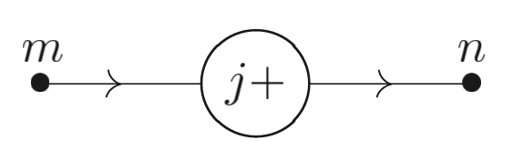
A Minsky machine is a super simple computer that has an infinite amount of memory in the form of registers each holding a non-negative integer, and exactly two types of operations, illustrated with the following pictures (taken from Nielsen, M. A., & Chuang, I. L. (2001). Quantum computation and quantum information (Vol. 2). Cambridge: Cambridge university press.):

The Inc operation adds 1 to the register named j:

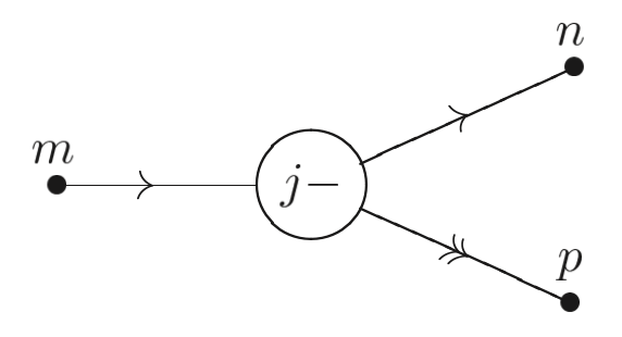
The Cdec (conditional decrement) operation subtracts 1 form the register named j and continues to point n, unless j==0, in which case it does nothing and continues to point p:

A program for a Minsky machine is a sequence of an arbitrary number of these two operations, which together form a graph. Typically there are also nodes between the operations which are named, and two special named nodes for the starting and halting states of the Minsky machine. Here is a very simple program with a slightly more compact visualization:

It moves the value from register 0 into register 1. We read it by starting at the first node² Cdec(r_0) and following the graph until we reach the HALT node. For the Cdec operation two outward arrows show the path that the program takes if the register is zero or non-zero (>0).

If we run the program on a set of registers (a, b), here is what we will get:

• (5, 0) -> (0, 5)
• (5, 3) -> (0, 8)
• (0, 5) -> (0, 5)

This program moves the value from the first register and adds it to the value in the second register. It something between a move and add operation in a typical programming language. In ARM assembly for example it would be equivalent to this program:

add r1, r1, r0
mov r0, #0

Here is what caught my attention: Notice how simple the Minsky machine is? It seems even simpler than the Turing machine, which has the moving head and arbitrary tape alphabets (though typically ${0, 1}$ is used). I know that a lot of different computational models ultimately turn out to be equally powerful (the Church-Turing thesis), but it is also often surprising why a particular model turns out to be equally powerful to all these other models. I remember that a couple of years ago, it was shown that the mov instruction on x86 systems is as powerful as a Turing machine, something that is called "Turing-Completeness". Proving that something is Turing-complete is something of a hobby for many people, and unusual things turned out to be Turing-complete. If you ever played Magic: The Gathering you might know that it is a complicated game, but it turns out that it is also Turing-complete! Funnily enough, since no computer can ever calculate whether an arbitrary computer program terminates or not (the famous Halting problem), this means that in principle, it is impossible to play perfect Magic.

So the task that the authors gave was this:

Show that Minsky machines are Turing-complete!

This is what I attempted over the past two weeks. The proof itself is not difficult (though it is satisfying to construct it), but I didn't want to stop there. I wanted to build a program that converts Turing machine descriptions into equivalent Minsky machines! That as it turns out took most of my time :)

Turing-completeness of Minsky machines - An idea

First I want to show the idea for demonstrating Turing-completeness of Minsky machines. It will illustrate why I found these machines to be so entertaining, because ultimately they behave like glorified LEGO bricks with which you can build more and more complex LEGO bricks. After that (probably in the next post) I'll show the program that I wrote for simulating Minsky machines and converting from Turing machines to Minsky machines.

We need a quick summary of the Turing machine (which you can read up on) before we can move onto the proof. This beloved (or hated, if you ask the average CS undergrad student) machine has infinite memory in the form of a tape made up of individual cells which hold a single value each. Typically we say that a cell holds either 0 or 1, as it can be shown that larger sets of tape symbols (called alphabets) don't make the Turing machine more capable (only faster, which we don't care about here). The Turing machine also has a tape head, which is a device that sits at some cell on the tape and can read and write its contents. A program for a Turing machine is then a sequence of instructions that take the current instruction (often called state) and the current symbol on the tape and, based on this, do three actions:

1. Write a new symbol 0 or 1 onto the tape
2. Move the tape head either left or right one cell
3. Go to a new state, which can be either any state with some fixed number, or a special state called HALT, which indicates that the machine is done

More formally, a Turing machine program is a list of entries of the form: $(q, S) \rightarrow (q', S', L/R)$ with:

• $q$: Current state
• $S$: Current symbol
• $q'$: New state
• $S'$: New symbol written to the tape
• $L/R$: Move tape head Left or Right

For completeness, here is the full program for a Turing machine called BB(3) (the 3-state Turing machine that produces the highest number of ones when starting with an empty type while still halting):

• $(A,0) \rightarrow (B, 1, R)$
• $(A,1) \rightarrow (C, 1, L)$
• $(B,0) \rightarrow (A, 1, L)$
• $(B,1) \rightarrow (B, 1, R)$
• $(C,0) \rightarrow (B, 1, L)$
• $(C,1) \rightarrow (HALT, 1, R)$

So how do we show that a Minsky machine is just as powerful as a Turing machine? At first glance, the two models look very different: The Turing machine has a single infinite tape made up of distinct ones and zeros, whereas the Minsky machine has an arbitrary number of integer-values registers. The Turing machine can move around the tape and manipulate individual bits, whereas the Minsky machine can only every add or subtract 1. And how do you even show that these two models are equally powerful?

One common way is to demonstrate that your desired model (the Minsky machine in our case) can simulate a Turing machine! By that we mean that we can take any Turing machine program and create an equivalent program for the Minsky machine that computes the same function³. Since a Turing machine is described fully by the tape contents, the position of the tape head, the current state and the state transition table, we need a way to simulate these four aspects on a Minsky machine. Let's start with the simplest one: The current state and state transition table.

1. Simulating Turing machine state transitions on the Minsky machine

You might notice that programs for the Minsky machine can be represented as directed graphs, as can programs for a Turing machine. This natural correspondence is a good starting point for building our Turing machine simulation on a Minsky machine. Each state in the Turing machine can be represented as a group of operations, with the state transition being a simple graph edge between the old state and the new state. For the BB(3) Turing machine, a corresponding graph looks like this:

Let's insert the action that the Turing machine performs on a state transition: The written symbol and the tape head movement. We can represent those as more nodes:

Notice how we end up with two differen types of nodes:

1. "Decider" nodes (displayed as ovals), which simply check for each state what the current symbol underneath the tape head is (0 or 1)
2. "Action" nodes (displayed as rectangles), which perform the state transition, write a new symbol and move the tape head (so (1,R) would write a 1 and move the tape head one position to the right)

The Decider nodes behave like an if/else statement, we will need to show that the Minsky machine is capable of performing such an operation. For the Action nodes, we first need to understand how to simulate the tape!

2. Simulating the Turing machine tape on the Minsky machine

Simulating the tape is a bit more tricky, and I'm sure there are more optimal ways of doing it than the one I chose. Working with an infinite tape seems daunting, until we realize that the Minsky machine registers are also infinite: There are an infinite number of them, and they store arbitrarily large natural numbers. You might be tempted to simulate the tape by assigning one register to each cell, maybe with some clever scheme where the cells to the left of the tape head use even indices and the ones to the right use odd indices. Unfortunately, the register specifiers in the ADD and Cdec operations of the Minsky machine are fixed in our program. We can't just say "Add 1 to the register specified by the value in this other register". In technical terms, the Minksy machine only supports direct addressing, not indirect addressing. So instead we can split up the tape into three sections, each represented by a single register:

Let's call those three registers L for the left side of the tape, R for the right side of the tape, and H for the single bit under the tape head. Since the tape stores a bit string, we can encode each of the three sections of the tape as a natural number using binary encoding. Notice though that L and R have different endianness, as the left section of the tape grows to the left, whereas the right section of the tape grows to the right. In the image, L would hold the little-endian value $110_2=6$ but R holds the big-endian value $BE(100_2)=001_2=1$! Splitting the tape into three sections seems to be a common construction, the Magic is Turing-complete paper uses the same idea.

Now we have the tape, all that is left is simulating tape head movements (writing a new value to the H register is trivial). We can do that by shifting the values in the L and R registers. If we move the tape head to the left, notice how the values in the registers change:

L is now little-endian $11_2=3$, R is now big-endian $0100_2=2$, and H remains zero. Mathematically, we can express this transformation with three equations applied in a specific order:

3. Initializing the tape

A typical setup for a Minsky machine would be to start with the input value $n$ in the first register and all other registers set to the value $0$: $(n, 0, 0, ...)$. The halting configuration would then have $f(n)$ in the first register (i.e. whatever function the machine computed) and again all other registers set to zero: $(f(n), 0, 0, ...)$ Since our construction uses three registers for the tape, we also need a way to initialize these three registers. Assuming our Turing machine tape starts at the leftmost bit of the input string, we can initialize the L, H and R registers like so, assuming $r_0$ holds the whole tape value:

L of course is zero by design. R holds all but the highest bit. For H we use a little trick. The highest bit of $r_0$ will never be zero unless $r_0$ is zero because we can disallow leading zeroes in the binary encoding of $n$ without changing the effective value of $n$. This makes the corresponding Minsky machine operations much simpler.

In the end we can combine L, H and R into the resulting value using string concatenation, which we can implement mathematically like so:

Let $s = \lfloor \log_2 R \rfloor + 1$ denote the bit-length of $R$. Then:

$r_0 = R + H \cdot 2^{s} + L \cdot 2^{s+1}$

Where to go from here

This concludes the construction of a simulation for a Turing machine using natural-number registers and simple mathematical operations. What remains to be shown is that we can implement all of these mathematical operations using a Minsky machine. I will cover this in the next part of this series, but to give an outlook, here is a list of all the operations that we are going to need:

• Adding two registers
• Multiplying a register by a constant
• Bit shifting the value in a register by a constant and by the value in another register
  • This is a special case of exponentiation, i.e. $r_a=c^{r_b}$
• Setting a register to zero or one
• Computing the remainder of a register divided by a constant
• A simple branching operation (do A if register value is zero, otherwise do B)
  • You might have noticed that this is basically what Cdec does :)

Stay tuned for the construction of all these operations, and an introduction to the simulation framework I wrote to actually run Minsky machines and test these operations!